My Journey from STAC APIs to Streaming SAR Imagery

How a simple catalog-browsing idea became a browser-based experiment in open imagery discovery

The Catalog Visibility Problem

There is a persistent visibility gap in the commercial imagery market.

The geospatial industry talks constantly about more satellites, more sensors, more collection capacity, and more data moving into cloud-native environments. At the same time, it remains surprisingly difficult for many analysts, researchers, students, journalists, and developers to visually explore what imagery actually exists.

Some of that complexity is natural. Commercial imagery is a business. Catalog access, licensing, tasking, archive search, fulfillment, and reseller relationships are all part of the value chain. Individual providers often have their own portals. Resellers maintain their own marketplace experiences. Enterprise customers may have custom interfaces or direct access agreements. For those inside the right workflows, the tools can be powerful. For everyone else, discovery can feel fragmented.

That fragmentation becomes even more noticeable when dealing with open, freely available imagery from commercial collectors. Open imagery plays an important role in the broader ecosystem. It gives developers test data. It gives educators real-world examples for explaining sensor capabilities. It gives journalists and researchers material they can use without going through a procurement process. It gives students and early-career professionals a way to learn from actual commercial data. During natural disasters, it can also help people quickly understand what has already been collected and what kinds of sensors may be useful for situational awareness.

Yet there are not many lightweight applications focused specifically on letting users browse open imagery catalogs on a map, inspect the available assets, and quickly understand what the data looks like before moving into heavier tools.

There are likely other STAC viewers and catalog browsers out there. I do not want to imply that I invented a new category of software or built something uniquely revolutionary. In fact, part of the truth is much less dramatic: I got curious, a little lazy, and wanted to create my own. I wanted something that fit the way I research, write, and explore geospatial data for Project Geospatial. Sometimes building a tool is less about inventing something entirely new and more about creating the version that matches your own workflow.

That is where the Umbra SAR Navigator started.

The Analyst Need Behind the Application

The original idea was simple. I wanted a quick way to see where open imagery data existed through STAC APIs across multiple providers.

As someone who writes about the industry, produces geospatial media, and spends a lot of time thinking about remote sensing capabilities, I often need to answer a basic question quickly: what open imagery exists over this location, from which collector, and what type of data is available?

I know how to use QGIS or ArcGIS. If I need to do more serious geospatial analysis, I can pull Cloud Optimized GeoTIFFs, STAC item assets, and other geospatial files into a desktop GIS environment. QGIS remains one of the best places to do real inspection and analysis. The challenge is that there are many moments when a full desktop GIS workflow is more friction than I need.

Sometimes I am working from a Chromebook. Sometimes I am preparing questions before an interview. Sometimes I am writing an article and need to quickly understand whether open imagery exists over a place. Sometimes I am exploring sensor capabilities and want to see the geographic footprint of a public dataset before downloading anything.

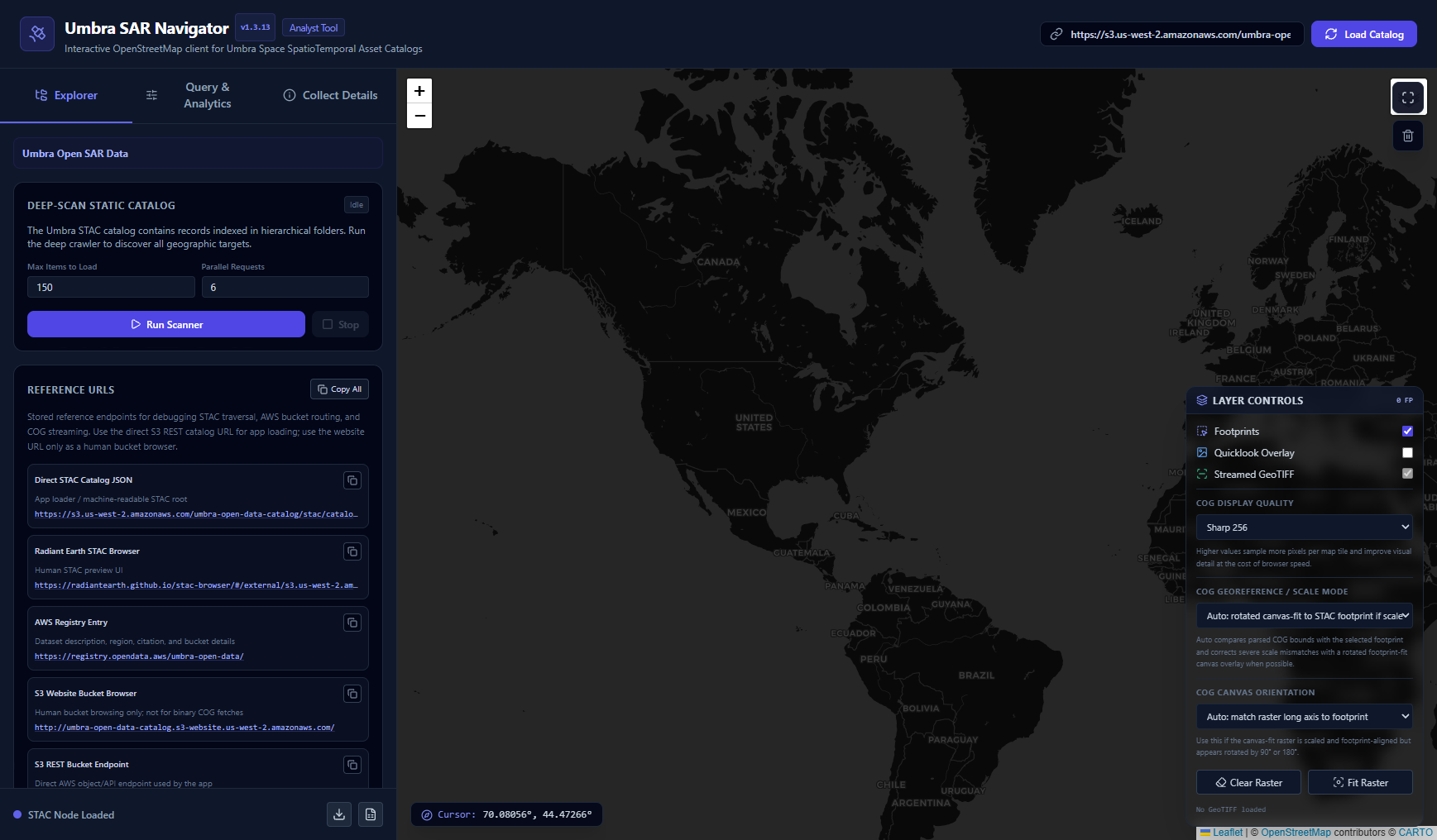
That practical need shaped the early requirements. The tool needed to run in a browser. It needed to be lightweight. It needed to work on GitHub Pages. It needed to let me paste or select a STAC URL, browse catalog items, display footprints, inspect deliverables, and view previews or imagery when possible.

The first serious test case became the Umbra Open Data Catalog.

Umbra’s open SAR data is a strong proving ground because it includes real Synthetic Aperture Radar collections, public STAC metadata, AWS-hosted assets, and multiple product types. A single collect may include a GEC GeoTIFF, SICD, SIDD, CPHD, metadata files, and quicklooks. That combination creates a useful but demanding test environment. The catalog is structured enough to build against, while the underlying data is complex enough to expose the weak points in a simple browser-based viewer.

Starting Small, Then Hitting Real Technical Friction

The first version of the application began in Gemini. I used it to rough out the initial development requirements and produce an early prototype. As the application grew, I moved more of the coding work into ChatGPT because it seemed to handle longer coding requests better, especially once the file crossed into several thousand lines of HTML, JavaScript, CSS, map logic, STAC parsing, analytics, and raster rendering behavior.

That shift became important as the project moved from basic catalog browsing into Cloud Optimized GeoTIFF streaming.

The early application could load the Umbra STAC catalog, show collection footprints, and display item metadata. That alone was useful. Seeing footprints on a map gave me the first part of what I wanted: a quick visual understanding of where open SAR collections existed.

The next question was whether the application could connect the STAC metadata to the actual files in the AWS bucket and stream the imagery directly into the browser.

That step became the major technical journey of the project.

On paper, the workflow sounds straightforward. A STAC Item points to assets. Those assets include links. Some of those links should point to image files. A Cloud Optimized GeoTIFF should be accessible over HTTP. A browser should be able to fetch it, parse it, and render it on a Leaflet map.

In practice, every part of that chain required debugging.

From STAC Metadata to Actual AWS Objects

The first major hurdle was asset discovery. A STAC item may contain several assets, and not every asset should be treated as a streamable raster. Some files are JSON metadata. Some are quicklook images. Some are NITF-based products better suited for QGIS or specialized tools. Some STAC metadata may be incomplete, inconsistent, or structured in ways that do not directly expose every file in the delivery folder.

The application needed to become more skeptical.

Loose filename matching was not enough. A naive search for “tif” could produce false positives. A MIME type alone was not reliable enough. Some URLs pointed toward S3 website-style paths rather than direct object paths. Some links led to HTML directory pages instead of binary files. Other cases required understanding how the STAC item related to the actual sar-data/tasks structure in the Umbra AWS bucket.

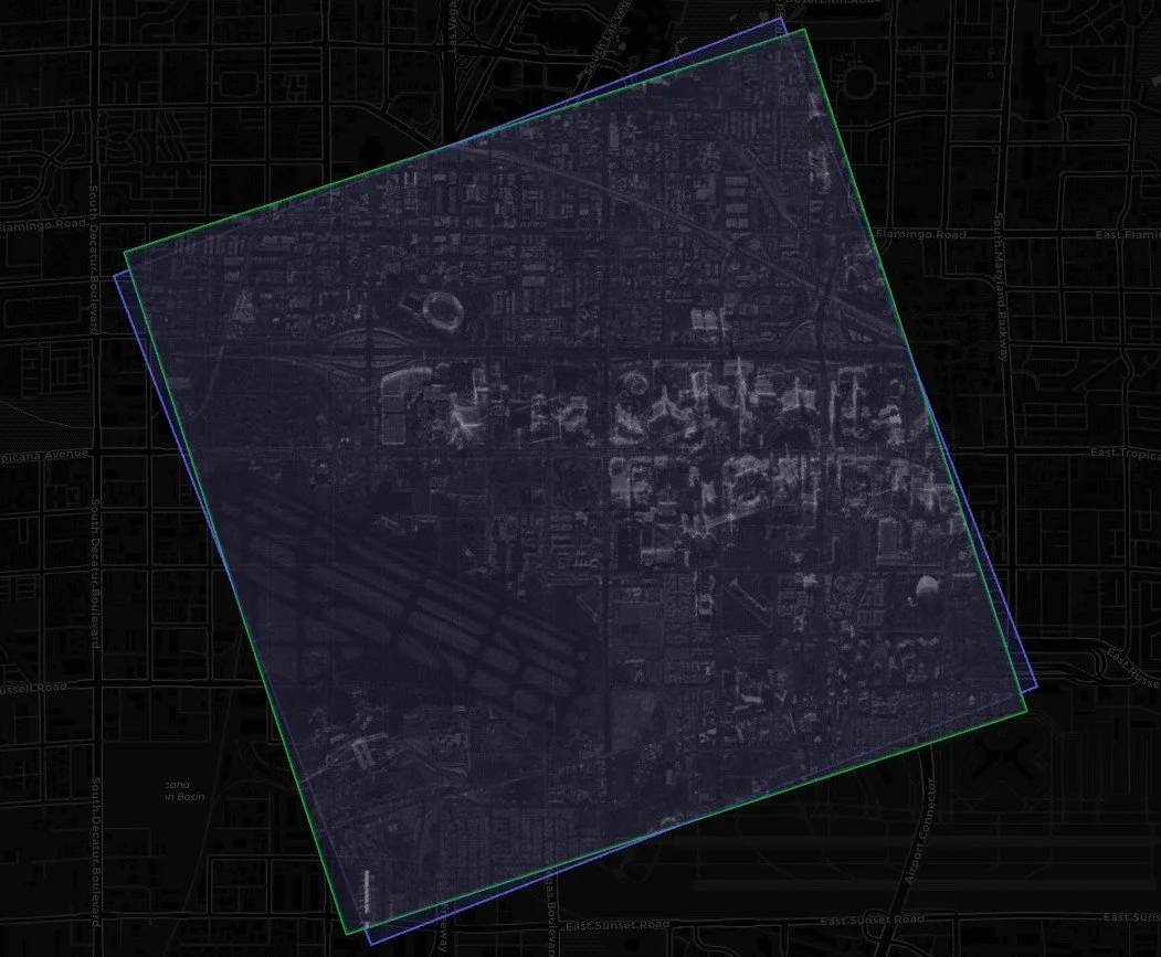
Connecting the STAC API to the physical files required building a more careful resolver. The app had to normalize S3 URLs, preserve encoded spaces and special characters in target names, identify collection IDs, derive or discover delivery folders, and prioritize the GEC .tif as the browser-streamable product. For the Las Vegas test images, this became especially clear. The working URL included the target name, collection ID, collect timestamp, satellite identifier, and _GEC.tif suffix. Missing or misplacing any part of that path produced a 404.

That part of the development process was a reminder that STAC is a powerful standard, but real-world catalogs still require practical interpretation. The metadata gets you close. The application still has to understand how a specific provider structures its public assets.

As the resolver improved, the application started finding and streaming the actual GEC GeoTIFFs. That was the moment the project became more than a catalog browser.

Streaming COGs in the Browser

Cloud Optimized GeoTIFFs are designed for cloud-native access. They allow clients to request pieces of a file efficiently rather than downloading and opening an entire raster in the traditional desktop GIS sense. For browser-based geospatial tools, that makes COGs especially attractive. They create a path toward lightweight imagery inspection directly from a web map, without requiring the user to first download a file, open QGIS, configure a raster layer, and manually inspect the scene.

Streamed COG within the browser, correctly oriented, scaled, and placed.

That was the theory. The practical implementation was more complicated.

The first challenge was simply making sure the application was connecting the STAC metadata to the correct file in the AWS bucket. A STAC Item may describe a collect and include links to several assets, but the browser still needs the exact object URL for the file it is going to stream. In the case of Umbra open data, that meant moving from the catalog record to the actual delivery folder in S3, identifying the correct collection ID, preserving encoded spaces in target names, and finding the GEC .tif file inside the collect folder. If any part of that path was derived incorrectly, the result was usually a 404 error from S3.

That part of the project became one of the bigger technical hurdles. The application had to learn the difference between a STAC catalog path and the real SAR data object path. It also had to handle the quirks of public S3 URLs, including website-style bucket links, direct object links, encoded characters, and folder structures that were not always obvious from the first catalog record. Once the app could reliably move from “this is the STAC item” to “this is the actual GEC GeoTIFF object in the bucket,” the streaming workflow became much more useful.

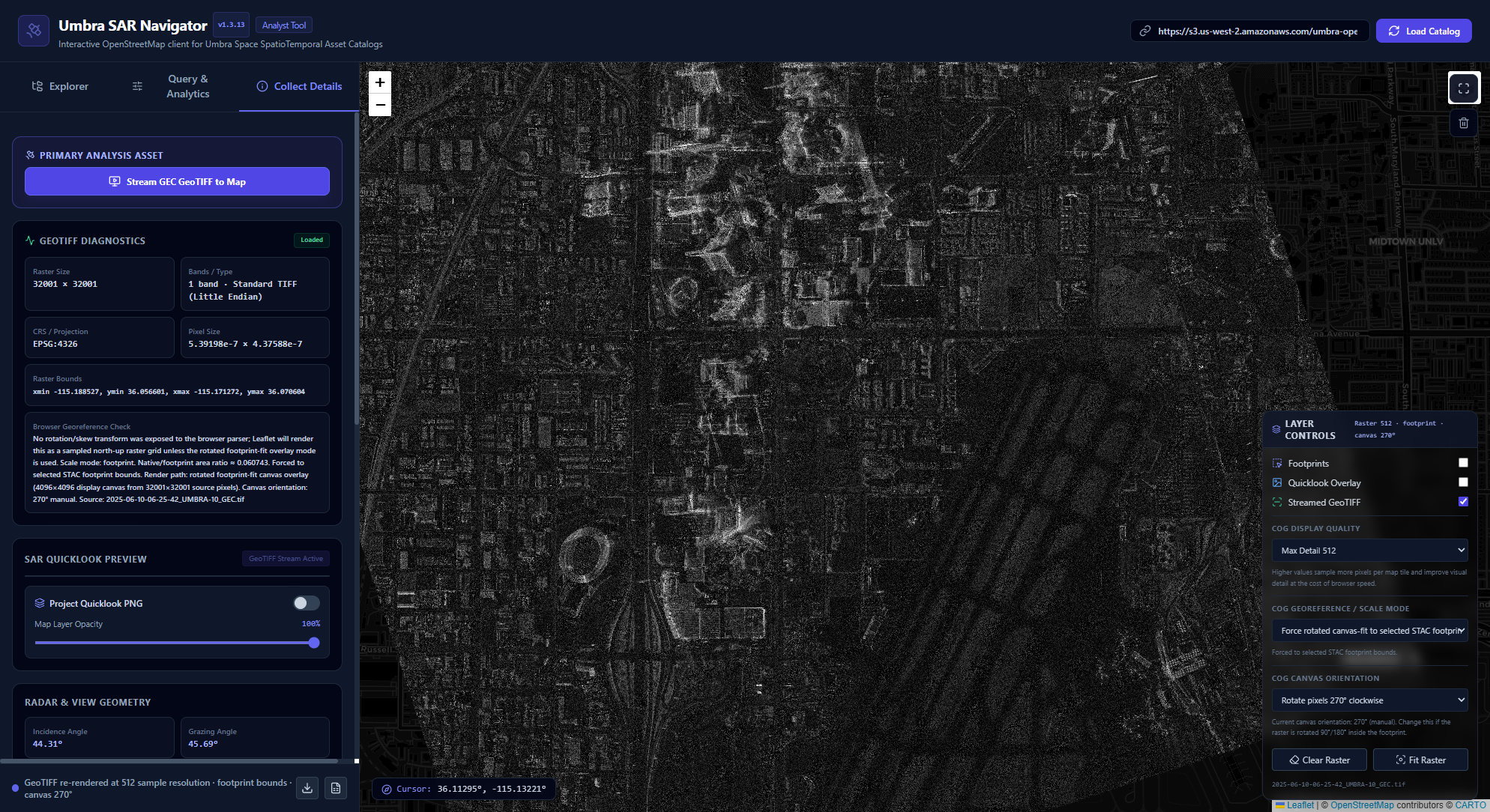
The next issue was validation. Before sending anything into the GeoTIFF parser, the application needed to confirm that it was actually receiving a TIFF. That sounds basic, but it matters. If the server returns JSON metadata, an HTML directory page, an XML error response, or a 404 page, a raster parser may fail in confusing ways. The application now checks the first bytes of the response before trying to render it. That gives the user a more understandable error when the file is not a valid TIFF, rather than letting the browser silently hang or throw a cryptic byte-order exception.

Once the app could reliably stream a GEC GeoTIFF, image quality became the next challenge. The first successful streams were exciting because the imagery was finally appearing in the Leaflet map. But the images initially looked softer than expected. The source data was not being degraded. The issue was the browser rendering configuration.

The map layer has to sample raster pixels for display. A lower sampling value makes the app faster and more responsive, but the image can look softer or more generalized. A higher sampling value improves visual clarity, but it increases the workload for the browser. That tradeoff matters because the application is meant to run in a lightweight environment, including laptops and Chromebooks, without a dedicated imagery server doing the heavy lifting.

That led to the COG display quality setting. The application currently gives users several options, including 256, 384, and 512.

The 256 setting is the practical default. It gives a sharper view than a low-resolution preview while keeping the browser reasonably responsive. For general exploration, 256 is usually the best starting point. It is useful when scanning through multiple scenes, checking whether a collect is interesting, or quickly comparing imagery against the footprint and basemap.

The 384 setting is a middle ground for users who want more detail without immediately pushing the browser to its heaviest mode. It samples more densely than 256, so features may appear clearer, especially in urban areas, ports, infrastructure sites, and high-contrast SAR scenes. The tradeoff is that panning, zooming, and rendering may feel slower depending on the size of the COG and the performance of the device.

The 512 setting is the high-detail browser mode. It pushes the rendering closer to the practical upper limit for this type of client-side viewer. It can make the streamed SAR image look noticeably sharper, but it also asks more from the browser. On a strong desktop machine, 512 may be useful for closer visual inspection. On a Chromebook or lower-powered laptop, it may introduce lag, longer render times, or a less responsive map. It is best used when the user has already selected a scene of interest and wants a better look, rather than when rapidly scanning through many images.

This quality control is important because it gives the user some control over the balance between speed and fidelity. A browser-based imagery viewer cannot assume every user has the same hardware, network connection, or patience for large raster rendering. The best setting depends on the task. If the goal is fast catalog exploration, 256 is usually enough. If the goal is closer visual inspection of one scene, 384 or 512 may be worth the extra wait.

There is also a distinction between display quality and source quality. Increasing the quality setting does not create new information in the image, and lowering the setting does not damage the source COG. The file remains the same. What changes is how densely the application samples and draws the raster into the browser map. That distinction is important because a soft-looking browser render can easily be mistaken for a low-quality image product when the real limitation is the client-side display pipeline.

The same lesson applied to the canvas-fit modes added later in development. When the app needed to correct scale or orientation issues, it sometimes rendered the SAR pixels into an intermediate canvas and then placed that canvas into the selected footprint. That approach made the imagery much more usable in the map, but it also meant the selected display quality influenced the size and clarity of the rendered canvas. Higher quality settings produce a more detailed canvas, but they also increase memory use and rendering time.

In practice, users should treat the quality setting as part of the workflow. Start with 256 when exploring the catalog. Move to 384 when a scene looks promising. Use 512 when you want the best browser-based view and are willing to wait for the render. If the app appears to be thinking, it probably is. These are real imagery files coming from a public cloud bucket into a client-side web application, not pre-rendered map tiles from an optimized imagery service.

That is one of the larger takeaways from the project. COGs make browser-based imagery exploration possible, but they do not remove every performance constraint. The browser still has to fetch, parse, sample, stretch, orient, and draw the raster. A lightweight app can make that process accessible, but it needs to expose enough controls for the user to manage the experience.

Scale, Rotation, and the Reality of Browser Georeferencing

After image quality, the next major challenge was scale.

At first, I assumed that if the application could successfully stream the GEC GeoTIFF, parse it, and place it on the map, the hard part was mostly over. That assumption did not last long. In several scenes, the image appeared dramatically smaller than the STAC footprint. This was not a minor offset. It was not the normal kind of SAR layover, foreshortening, or terrain-related displacement an analyst might expect from radar imagery. The raster could appear as if it were only a tiny fraction of the collection area, almost like it had been shrunk down inside the footprint.

That was an important distinction. The app was not failing to read the file. The pixels were there. The COG was streaming. The browser was parsing enough of the raster to display an image. The problem was that the browser rendering layer was not placing the raster at the same scale as the STAC footprint.

This is where the difference between “the catalog footprint” and “the raster’s parsed georeference” became important.

The STAC footprint gives a geographic polygon for the collect. It is the catalog’s description of where the scene is located on the Earth. The GeoTIFF also carries geospatial information, but in a lightweight browser environment, that information may be parsed or interpreted differently than it would be in a full GDAL-based workflow. The browser library may expose simple bounds, pixel size, coordinate reference information, and raster dimensions, but it may not always handle every transformation nuance the same way a desktop GIS would.

In practice, that meant the application had two competing sources of geospatial truth: the STAC Item footprint and the GeoTIFF’s parsed native bounds. When those two agreed reasonably well, the native rendering path could work. When they disagreed dramatically, the browser needed a fallback.

The first step was to make the mismatch visible. I added a georeference diagnostic check that compared the native GeoTIFF bounds against the selected STAC footprint. The app calculated a rough area ratio between the two. In some cases, that ratio made the problem obvious. The native raster footprint could be a tiny percentage of the STAC footprint. When the app reported something like a native-to-footprint area ratio of 0.0005, it was a clear sign that the browser render path was not placing the image correctly.

That diagnostic changed the development approach. Rather than trying to pretend the parsed bounds were always correct, the app could make a decision: use the native GeoTIFF bounds when they looked reasonable, or switch to a footprint-fit mode when the mismatch was severe.

The first footprint-fit mode was conceptually simple. The application rendered the SAR pixels into a browser canvas, converted that canvas into an image overlay, and placed the overlay inside the selected STAC footprint bounds. This physically stretched the rendered SAR image into the geographic area described by the STAC item. It was a practical solution to the scale problem because it stopped relying on the browser’s native GeoTIFF placement when that placement was clearly wrong.

That approach worked better than trying to force the GeoTIFF layer itself into new bounds. In earlier tests, simply passing footprint bounds into the raster layer did not always fix the visual scale problem, because the rendering layer could still behave according to the parsed native raster coordinate model internally. The canvas-fit approach was more direct. It said, in effect: render the pixels first, then place that rendered image into the footprint.

For a lightweight browser viewer, that was a useful breakthrough.

It also required a philosophical decision about what the application was trying to accomplish. The purpose of this tool is rapid discovery, inspection, and education. It is meant to help a user see where open SAR imagery exists, inspect the available files, and get a practical look at the image in context. It is not trying to replace a professional exploitation workflow. Once that purpose is clear, a footprint-fit mode becomes reasonable. It is a visualization aid that helps align the image with the catalog footprint when the browser’s native georeferencing path is not reliable enough.

The next issue was that fitting the image into the footprint as a north-up rectangle still did not always look right.

SAR collection footprints are often angled. The collect geometry may be a rotated polygon rather than a simple rectangular box aligned to north. If the application stretched the image into a normal Leaflet bounding box, the scale could improve while the orientation remained wrong. The image would occupy the right general area, but it would not follow the direction of the footprint.

That led to the rotated footprint-fit overlay.

Instead of placing the rendered SAR canvas into a standard north-up rectangle, the app attempts to derive usable corners from the STAC footprint polygon. It then uses those corners to orient the canvas overlay along the footprint’s geometry. In simple terms, the image is no longer only being stretched into the footprint’s bounding box. It is being rotated to follow the footprint’s edge direction.

That improved the visual alignment significantly. The image could now scale into the footprint and rotate with the collection geometry. For many scenes, that made the streamed COG much more useful in the browser.

But rotation introduced another subtle problem: the canvas itself might be oriented the wrong way before it is placed into the footprint.

The application has to decide which edge of the rendered raster corresponds to which edge of the footprint. If the raster’s pixel axes are effectively swapped relative to the footprint, the overlay can be rotated to the correct footprint angle but still show the image turned 90 degrees, 180 degrees, or 270 degrees from the expected visual orientation. This is why the app eventually needed a canvas orientation control.

That control gives the user a practical way to rotate the rendered SAR pixels before they are fitted into the footprint. The options include source orientation, 90 degrees clockwise, 180 degrees, and 270 degrees clockwise. There is also an auto mode that attempts to match the raster’s long axis to the footprint’s long axis. This is not a perfect solution, but it gives the analyst a way to correct the most obvious orientation mismatch without leaving the browser.

The sequence of fixes became a useful lesson in browser-based geospatial visualization:

• First, the app had to stream the COG.

• Validate the COG.

• Render the COG at a useful quality.

• Detect when the browser’s native georeferencing was not matching the STAC footprint.

• Fit the rendered pixels into the footprint.

• Rotate that fitted overlay to match the footprint geometry.

• Allow pixel-axis orientation corrections when the rendered image was turned the wrong way.

Each step solved one layer of the problem and exposed the next.

This may sound like a lot of manual correction for a simple viewer, and in some ways it is. But it is also an honest reflection of the gap between lightweight browser rendering and professional geospatial image handling. A full desktop GIS or GDAL-backed image service has a much deeper geospatial rendering stack. It can handle projections, transformations, resampling, warping, and georeferencing with more authority. A single-page browser application has to work with what JavaScript libraries can parse, what the browser can render, and what the user’s machine can handle.

That is why the application now exposes these controls rather than hiding them. The user can choose native GeoTIFF bounds when the raster places correctly. They can choose canvas-fit when the scale is wrong. They can use rotated footprint-fit when the image needs to follow the collection geometry. They can adjust canvas orientation when the image appears turned the wrong way. The diagnostics help explain which render path is being used and why.

For an analyst, that transparency matters. A bad visualization can be worse than no visualization if the user assumes it is precise. By exposing the render mode, scale behavior, and orientation options, the application makes it clearer that this is a browser-based inspection tool. It is meant to help users quickly explore open imagery and understand what they are looking at. When exact measurement, exploitation, or geospatial precision is required, the appropriate next step is still QGIS, a GDAL workflow, or a server-side tiling and reprojection service.

For my purposes, the viewer became useful once it could stream the data, detect severe scale mismatch, fit the image into the STAC footprint, rotate it to follow the footprint geometry, and let the user correct obvious pixel orientation issues. That combination turned the application from a simple catalog browser into a practical open imagery inspection tool.

The technical journey also reinforced one of the broader lessons of the project: open imagery access is not only about making files public. The data also needs usable pathways for discovery, streaming, visualization, and interpretation. STAC and COGs provide much of the foundation, but lightweight applications still have to bridge the last mile between metadata, cloud storage, browser rendering, and analyst understanding.

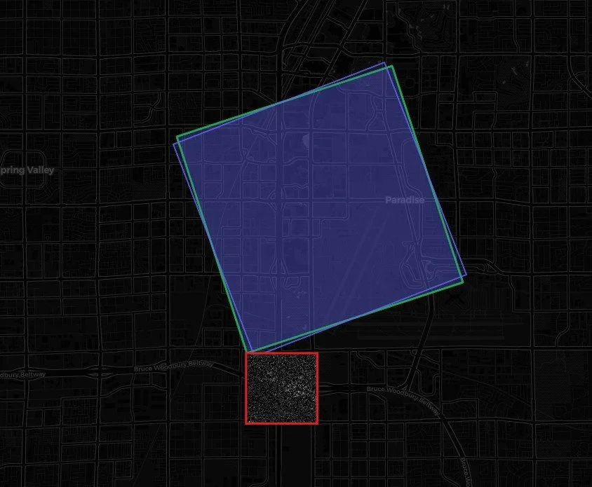
Example of the COG loading but not scaled, oriented, or placed correctly on the map

COG fitted to the footprint, but not oriented correctly

COG fitted to the footprint, scaled and oriented

Adding Analytics to the Viewer

Once the core browsing and streaming workflow started working, the next step was analytics.

Seeing a single image is useful. Understanding the shape of the catalog is more valuable. The application now includes geographic analytics that summarize loaded collections by country, state or region, date range, incidence angle, platform, polarization, and product type. These analytics are intentionally lightweight and client-side. They are not a replacement for authoritative boundary intersection or a full spatial database. They do, however, help answer practical questions quickly.

Where are the collections concentrated? Which regions appear most often? What product types are represented? What does the temporal spread look like? How much of the catalog has streamable imagery versus metadata or preview-only assets?

Those questions matter for open imagery catalogs because the value of the dataset is not only in individual scenes. It is also in the distribution of the archive. For educators, that distribution helps identify examples. For journalists, it helps support research. For developers, it helps locate test data. For analysts, it helps characterize what a collector has chosen to release publicly.

This is especially relevant for natural disaster workflows. During a flood, hurricane, wildfire, earthquake, or other crisis, the first question is often whether relevant imagery already exists. A lightweight map viewer with basic analytics can help users understand what is available before they decide whether to move into deeper tools or request additional data.

A Note for Users: Be Patient with the Data

One practical note for anyone testing the application: be patient with the loading process.

The scanner is walking a public STAC catalog and checking cloud-hosted assets, so it can take some time for footprints, deliverables, and analytics to populate. The same is true when streaming a GEC GeoTIFF into the viewer. These are real imagery files coming from an AWS bucket, and depending on the file size, browser performance, network conditions, and selected display quality, downloading and rendering a COG can take a few minutes.

The best approach is to let the scanner finish, select one image at a time, and avoid getting too click-happy while the app is fetching or rendering data. This is still a lightweight browser experiment, not a fully optimized enterprise image service. If the interface seems like it is thinking, it probably is.

A Humble Open-Source Experiment

The current version of the Umbra SAR Navigator is available on GitHub Pages. I encourage people to check it out, test it, break it, and send feedback. It is an open-source experiment, not a finished enterprise product and it still has a some quirtks

I encourage people to check it out, test it, break it, and send feedback. It is an open-source experiment, not a finished enterprise product. The current working version remains a single HTML file, which makes it easy to share and deploy. That simplicity has been helpful during rapid iteration, although it is already pushing the limits of maintainability.

I also have a more stable multi-file variant in progress. That version is designed to separate the application into supporting files, provider-specific logic, configuration, and reusable modules. That architecture will matter as the project grows beyond the Umbra Open Data Catalog and becomes more generalized for other STAC APIs.

That future direction is important. Umbra is the test case, but the broader idea is a provider-agnostic open imagery viewer. Some providers may expose full COGs. Others may only expose previews, thumbnails, or metadata. A useful STAC viewer should handle that range gracefully. It should show what is available, explain what can be streamed, and make the catalog easier to understand.

There are likely better STAC viewers, more complete catalog tools, and more technically sophisticated approaches already available. I built this one because I wanted to learn, because I wanted something lightweight for my own research, and because AI-assisted development made it possible for me to turn an analyst workflow frustration into a working prototype.

AI-Assisted Development from an Analyst’s Perspective

I am not a developer by trade. I am a geospatial analyst, media producer, consultant solutions strategist, and industry observer who has spent years around imagery, remote sensing, GEOINT workflows, and the commercial geospatial market. I know enough technically to understand what I want, test whether it works, and recognize when the output is wrong.

That combination is becoming increasingly powerful.

AI-assisted software development allows analysts to build tools closer to the shape of their own problems. It does not remove the need for technical understanding. In some ways, it increases the need for it. AI can generate code, but the analyst still has to know when a STAC link is pointing to the wrong object, when a raster is mis-scaled, when a COG is rendering at low quality, or when a SAR image is visually misleading.

The development of this application reinforced that point repeatedly. The hard part was not simply getting code to run. The hard part was connecting domain knowledge to implementation: understanding STAC, S3, SAR product types, COG behavior, browser rendering, catalog structure, and the practical needs of imagery discovery.

That is the part I found most rewarding.

Making Open Imagery Easier to Explore

The geospatial industry has invested heavily in better sensors, better APIs, better cloud infrastructure, and better data formats. The next step is making those capabilities easier to discover and understand.

Open commercial imagery has enormous value for education, research, journalism, disaster awareness, and software development. But that value depends on accessibility. People need simple ways to see what exists, where it exists, what files are available, and what the data looks like.

The Umbra SAR Navigator is my small contribution to that problem. It began as a personal tool for exploring open imagery catalogs from a browser. It became a learning exercise in STAC, AWS object paths, COG streaming, SAR visualization, and AI-assisted development. It is still evolving, and it still has rough edges. But it already demonstrates that an analyst with a clear workflow need can build something useful in this new era of software creation.

If you work with STAC catalogs, open imagery, SAR data, disaster response, geospatial education, or browser-based mapping, I would love for you to try it and share your thoughts:

https://wildcardspades58.github.io/umbra-sar-navigator/

The more people experiment with open imagery tools, the better the ecosystem becomes. For an industry that often talks about democratizing access to geospatial data, making the catalogs easier to see is a practical place to start.